No label? Make one!
You may remember one of the best paper at this year ICLR: rethinking generalization: even if the training images are assigned to random labels, the network can still get 0 training error. So, what if we use random labels to train a network, then use the learned features to do other tasks?
Unsupervised Learning by Predicting Noise is basically trying this idea. They train a network to predict noise, and then use the feature to do other tasks. Since there is no need for any labels, this is an unsupervised learning method.
Method:
The general supervised learning is: suppose we have n samples \(x_i\), and each sample has a target \(y_i\)(not limited to a class), we have to learn a function \(f_\theta\), so that expected loss is minimized,
\[\min_\theta \frac{1}{n}\sum l(f_\theta(x_i),y_i)\]However, in the case of unsupervised learning, we do not have this target \(y_i\), so what should we do? The answer is learn the \(y_i\). So our objective now becomes:
\[\min_\theta \frac{1}{n}\min_{y_i}\sum l(f_\theta(x_i),y_i)\]However, if we don’t put any constraints on \(y_i\), we will get a trivial result: all \(y_i\)s are constant, then \(f_\theta\) outputs this constant all the time.
In order to avoid this issue, the authors choose k representations in advance (k must be larger than n; these k representations are fixed), and then \(y_i\) must be selected from the k representations, and the same representation can only be chosen by one\(y_i\).
If we denote in matrix form, then the target \(Y\) is a \(n \times d\) matrix (each line is \(y_i\) and d is the length of y), \(C\) is a \(k \times d\) matrix, containing pre-selected k representations.
Then \(Y = PC\),
P is a \(n \times k\) assignment matrix, with values of 0,1. If \(P (i, j)\) is 1, then \(y_i = C_j\). And \(P\) must satisfy that \(P1_k \leq 1_n\), \(P^\intercal 1_n = 1_k\). (This is the mathematical form of the above selection constraint)
So the training objective becomes
\[\min_\theta \min_P l(f_\theta (X), PC)\]Details:
Loss: l2 distance
\(f_\theta (x)\): outputs a unit vector of length d
C: uniformly sampled from the unit sphere
In nutshell, this algorithm is finding a network that could map all the training data to a unit sphere uniformly.
Algorithm:
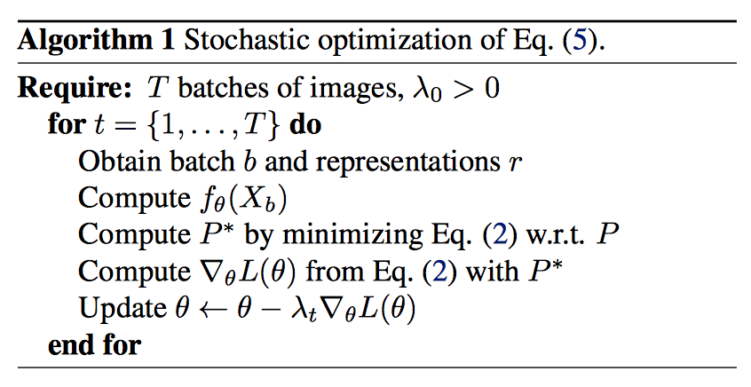
The algorithm is kind of similar to k-means. First, given current parameters, find new assignment \(P\), and then fix the new assignment to optimize \(\theta\).
However, due to the size of data, they use the sgd method. For the assignment, they only update the sub-matrix of the current batch, that is, the change of assignments can only occur inside the batch.
Implementation details:
Network structure: alexnet
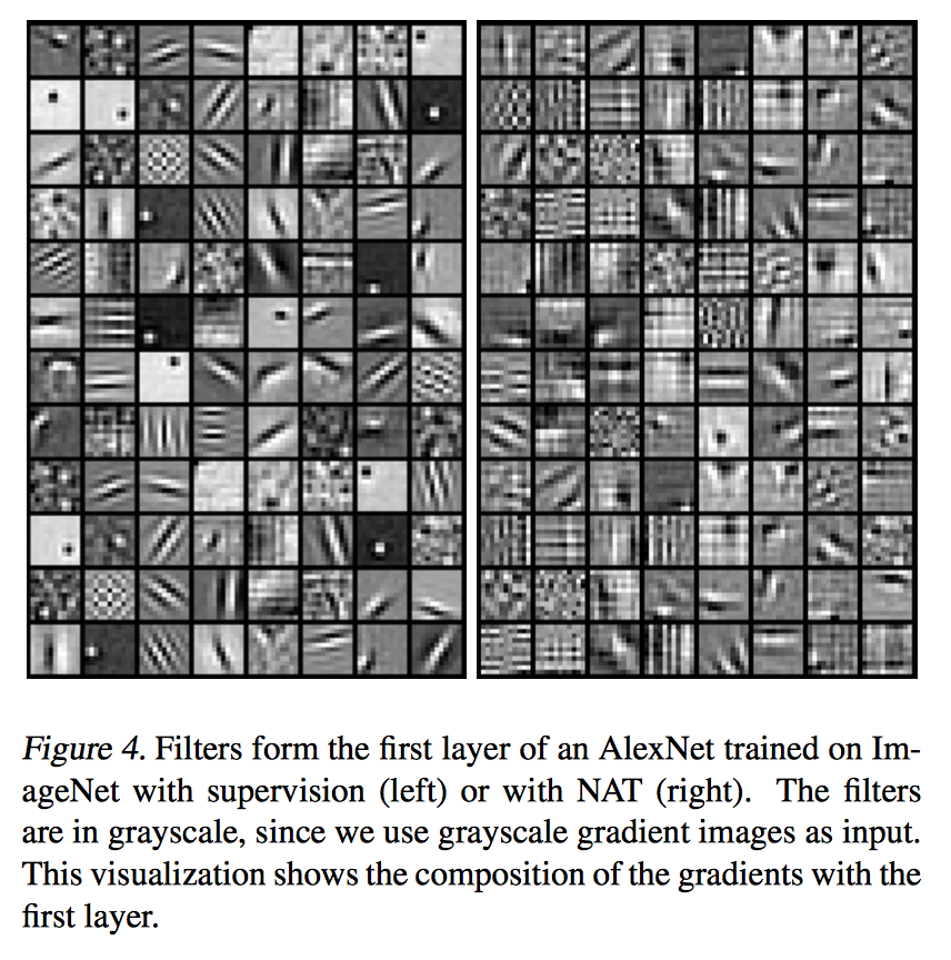
Preprocessing: they do not use raw image as network input because it will lead to trivial clustering by color. They use gray scale image gradient. In addition, they adopt commonly used data augmentation methods like flip, crop.
Experiment Setup:
Pretrain the cnn using this algorithm; fix the cnn, and finetune on image classification and detection tasks.
Ablation study:
Softmax vs square loss: They compared the difference between the softmax loss and the l2 loss on the image classification problem, and found that the gap was small, so l2 is suitable loss.
Preprocessing: Using grayscale gradient can improve the results of unsupervised methods, but they also found that it did not lose too much information.
Continuous vs discrete representation: If you use discrete representation, it is similar to k-means clustering, which is assuming all the samples can be divided into k categories. The author tried and found the result is much worse than the continuous.
Evolution of features: the more you pretrain using unsupervised training, the better the transfer ability.
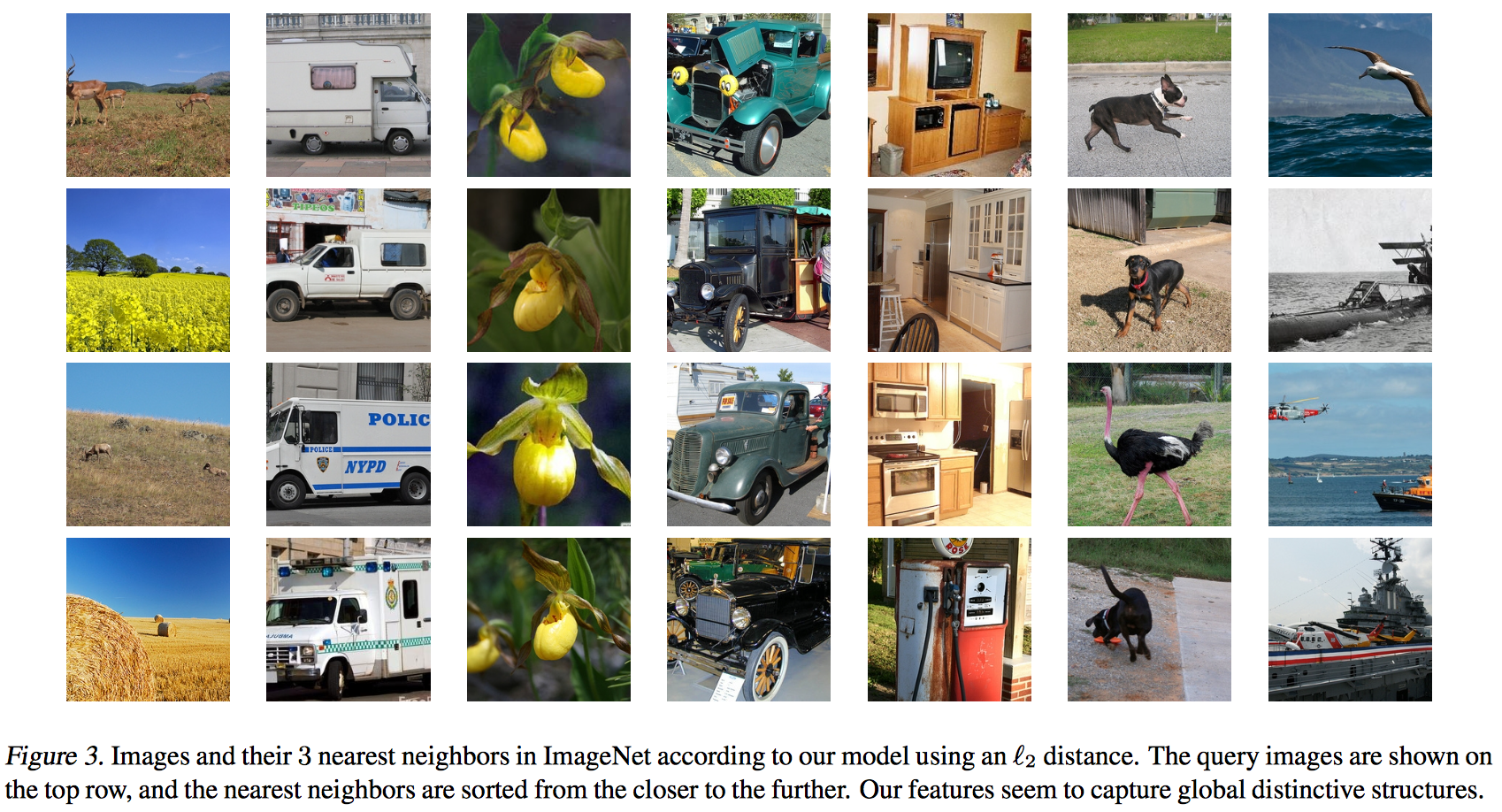
Nearest Neighbor Search:
Filter visualization:
Quantitative results:
Imagenet classification: this method is slightly better than BIGAN which is also an unsupervised method. They also compare to some self-supervised methods, among which some are better and some are worse. However self-supervised methods have to design the self-supervision task based on the problem setting, however the method in this paper is universal.
However, they also compared to the hand-crafted SIFT + Fisher vector, and found that the result of this paper is far worse.
Pascal voc: they compared the transfer ability of the network from imagenet to pascal. They found that this method is much better than autoencoder or normal GAN, and is slightly better than BIGAN.
Conclusion:
Interesting.